
Histogram Layers for Texture Analysis
Problem Statement: Shortcomings of Convolutional Neural Networks
Convolutional neural networks (CNNs) have shown tremendous ability for a variety of applications. One reason for the success of CNNs are that they excel at representing and detecting structural textures. However, they are not as effective at statistical textures. To illustrate this point, below is an example of different structural and statistical textures:
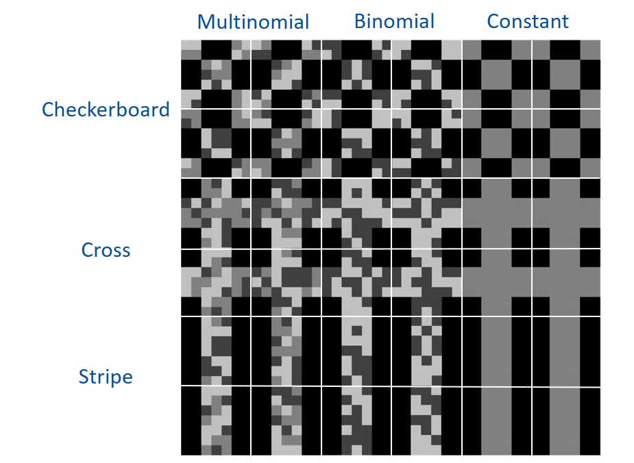
We can visually see the distinct differences between the different texture combinations. The structural textures are a checkboard, cross, and stripe. The statistical textures are shown through foreground pixels values sampled from multinomial, binomial, and constant distributions. A CNN could easily distinguish the structural textures, but would struggle with the statistical textures.
Why would a CNN struggle with statistical textures?
Structural texture approaches consist of defining a set of texture examples and an order of spatial positions for each exemplar (Materka et al., 1998). On the other hand, statistical texture methods represent the data through parameters that characterize the distributions and correlation between the intensity and/or feature values in an image as opposed to understanding the structure of each texture (Humeau-Heurtier, 2019). To understand differences between these two texture types, we created an example using the three distributions discussed above to generate statistical textures: multinomial, binomial, and constant classes. The first statistical class was sampled from a multinomial distribution with the following three intensity value choices which were of equal probability (p = 1/3): 64, 128, and 192. For the second statistical class, a binomial distribution (p = .5) was used where either an intensity value of 64 or 192 was selected for each foreground pixel. The last statistical class only contained foreground pixels with an intensity values of 128. Below we show the distribution of foreground pixel intensities after several trials (n=1800) and observe the means are the same.

A convolution is a weighted sum operator that uses spatial information to learn local relationships between pixels. Given enough samples from each distribution, the mean values are approximately the same and outputs from a convolution will be similar. We show example images convolved with a random convolution and observe the outputs are close in value. After many images are generated, the distribution of convolution outputs are similar as shown:
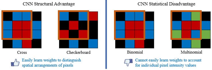
The average operation is a special case of convolution where all the weights are equal to 1/number of data points. As a result, the CNN will struggle to capture a linear combination of pixels that learns the statistical information of the data (i.e., cannot easily learn weights to discriminate statistical exemplars). Here is an example where if a 3x3 convolution is used, the model can easily learn weights to tell the cross and checkboard apart. However, if we sample from a different distribution and retain the same shape, a convolution operation cannot learn weights to distinguish this change as the convolution is unable to account for individual pixel intensity changes.
In summary, CNNs are great at structural texture changes. However, for statistical textures, CNNs fail to characterize the spatial distribution of features and require more layers to capture the distributions of values in a region.
Method: Histogram Layer
Standard Histogram Operation
The proposed solution is a local histogram layer. Instead of computing global histograms as done previously, the proposed histogram layer directly computes the local, spatial distribution of features for texture analysis, and parameters for the layer are estimated during backpropagation. Histograms perform a counting operation for values that fall within a certain range. Below is an example where we are counting the number of 1s, 2s, and 3s in local windows of the image:
Radial Basis Function Alternative
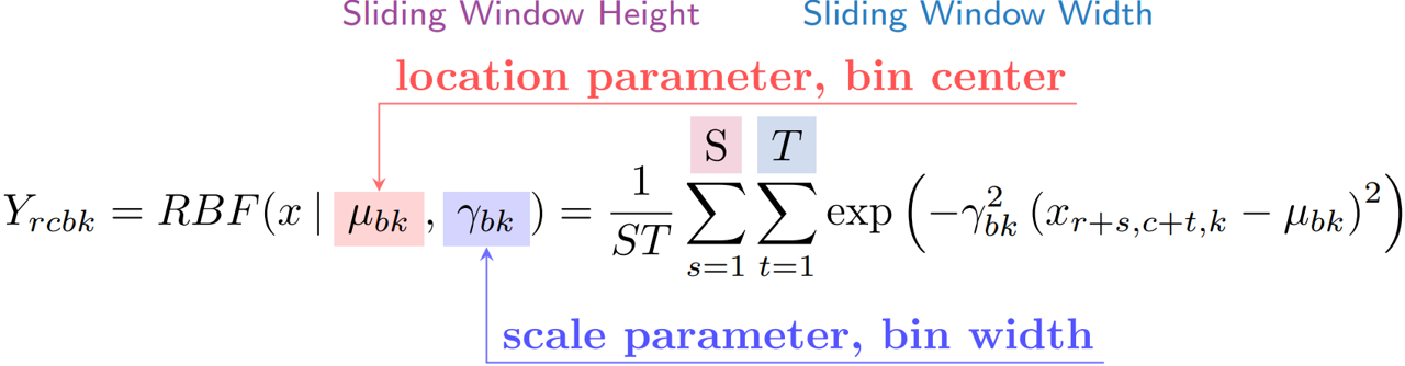
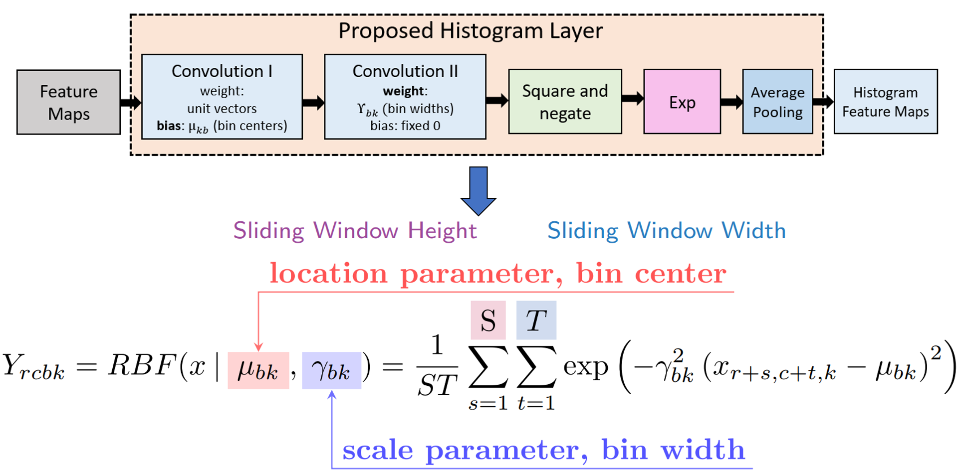
The standard histogram operation is not differentiable and is brittle (i.e., sensitive to parameter selection). However, a smooth approximation (i.e., radial basis function or RBF) can be used and the parameters (i.e., bin centers and widths) are updated via backpropagation. RBFs have a maximum value of 1 when the feature value is equal to the bin center and the minimum value approaches 0 as the feature value moves further from the bin center. Also, RBFs are more robust to small changes in bin centers and widths than the standard histogram operation because there is some allowance of error due to the soft binning assignments and the smoothness of the RBF. The means of the RBFs (μbk) serve as the location of each bin (i.e., bin centers), while the bandwidth (γbk) controls the spread of each bin (i.e., bin widths), where b is the number of histogram bins and k is the feature channel in the input feature tensor. The normalized frequency count, Yrcbk, is computed with a sliding window of size SxT, and the binning operation for a histogram value in the kth channel of the input X is defined as:
We show an example of the local operation of the RBF with a 3x3 window (S,T = 3), 1 input channel (K = 1), and three bins (b = 3) below:
Implementation of Histogram Layer
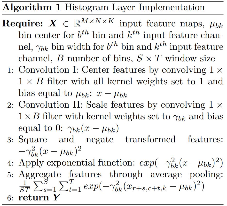
Another advantage of the proposed method is that the histogram layer is easily implemented using pre-exisiting layers! Any deep learning framework (e.g., Pytorch, TensorFlow) can be used to integerate the histogram layer into deep learning models. We show the configuration of the histogram layer using pre-existing layers and psuedocode below:
Applications of Histogram Layer
There are several real-world applications for the histogram layer! Statistical texture approaches are vital because there are important properties these methods inherit. For the histogram layer, the proposed method is globally permutation and rotationally invariant. If applied to smaller spatial regions, the operation is permutation and rotationally equivariant. As a result, the local operation is not sensitive to the order of the data and is robust to image transformations such as rotation. Additionally, the histogram layer is also translationally-equivarient (just like CNNs). Examples of usefulness of these properties include automatic target recognition (Frigui and Gader, 2009), remote sensing image classification (Zhang, et. al., 2017), medical image diagnosis (Bourouis, et al., 2021), and crop quality management (Yuan, et. al., 2019).
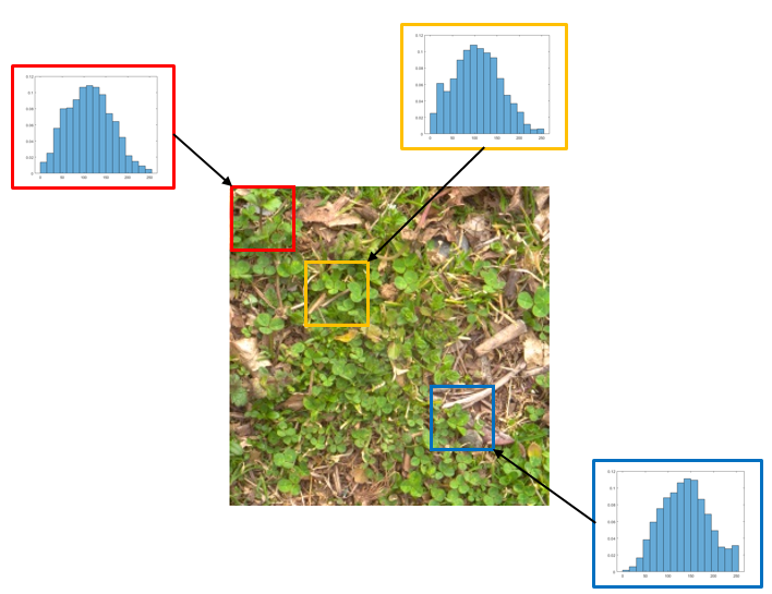
This is an example image of grass from GTOS-mobile. The image contains other textures and not only grass. Local histograms can distinguish portions of the image containing pure grass (top two histograms) or a mixture of other textures (bottom histogram) despite structual similarities. The histograms shown here are the distribution of intensity values from the red, green, and blue channels. Each histogram contains the aggregated intensity values (over the three color channels) in the corresponding image portion.
Histogram Layers for Synthetic Aperture Sonar Imagery
Synthetic aperture sonar (SAS) imagery is crucial for several applications, including target recognition and environmental segmentation. Deep learning models have led to much success in SAS analysis; however, the features extracted by these approaches may not be suitable for capturing certain textural information. To address this problem, we presented a novel application of histogram layers on SAS imagery (Peeples, et. al., 2022). The addition of histogram layer(s) within the deep learning models improved performance by incorporating statistical texture information on both synthetic and real-world datasets. We show an example below using the Pseudo Image SAS (PISAS) dataset.
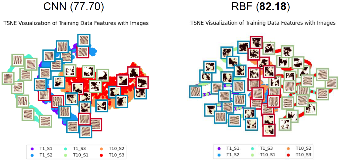
t-SNE projections for the convolutional and histogram layer models on the PISAS dataset. The overall test classification accuracy is shown in parenthesis. Example images from each class are shown. The structural classes are sand ripple (“T1”) and rocky (“T10”). The frames around each image represent the statistical class of the PISAS dataset. Red, green, and blue frames represent the multinomial, constant, and binomial distributions respectively. The CNN model appears to map structural textures near one another in the projected space (i.e., sand ripple images are grouped to the left region of the projection and the rocky textures are grouped in the right of the projection). On the other hand, the histogram layer model maps statistical textures close to one another. The binomial statistical textures (blue frames) are grouped in the left of the projection. The multinomial (red frames) and constant (green frames) statistical textures are clustered in the center and right of the projection respectively.
Check Out the Code and Paper!
This work was accepted to the IEEE Transactions on Artificial Intelligence! Our code and paper are available!
Citation
Plain Text:
J. Peeples, W. Xu and A. Zare, “Histogram Layers for Texture Analysis,” in IEEE Transactions on Artificial Intelligence, vol. 3, no. 4, pp. 541-552, Aug. 2022, doi: 10.1109/TAI.2021.3135804.
BibTex:
@Article{Peeples2022Histogram,
Title = {Histogram Layers for Texture Analysis},
Author = {Peeples, Joshua and Xu, Weihuang and Zare, Alina},
Journal = {IEEE Transactions on Artificial Intelligence},
Volume = {3},
Year = {2022},
number={4}
pages={541-552}
doi={10.1109/TAI.2021.3135804}}
Links


![]()